Take a line of unit length and remove the piece between 1/3 and 2/3. The two remaining pieces are 1/3rd the length of the original. We can think of each as being a smaller image of the original line and again remove the middle third of these two pieces. This leaves us with 4 identitcal lines each 1/3*1/3 = 1/9th of the original piece. The process doesn’t affect the end points of each line, and repeat this middle-third removal ad-infinitum and you end up with a set of infinitely many points, the ‘Cantor dust’.

This, the middle-thirds Cantor set, is a famous mathematical object. After infinite steps the set has uncountably many points but no length. The original definition of fractional dimension was devised to capture a property of similar sets that were ‘large’, in the sense of being infinite in number, and dense, but that still had no volume or length. The first proposed measure of these sets was the Hausdorff dimension which takes on integer amounts for relatively smooth objects like lines and cubes but fractional amounts for ‘rough’ objects like the Cantor set. The cantor set also has the property of being self-similar, each iteration is a scaled image of the previous set. This latter property is one associated with fractal objects and one reason why the term ‘fractal-dimension’ is commonly used in place of ‘fractional-dimension’.
While the origins of the term are interesting, it seems to also have added an unnecessary air of mystery to the idea of fractal dimension. In the this post I try to demonstrate that fractal dimension is a statistical property that relates to fundamental properties of the graph of a time series or random processes. In particular, fractal dimension can be described in terms of the autocorrelation function of a time series. Changes in fractal dimension can also be readily seen in the graphs of time series or random fields.
(If you are interested in more mathematical details, this post is based on a nice and not too long paper by Tilmann Gneiting.
Autocorrelation Function (ACF)
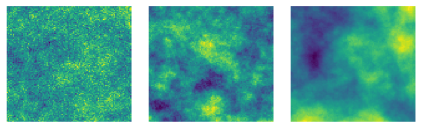
Informally, the fractal dimension of a time series measures a relation of points that are close to each other. An increase in fractal dimension corresponds to an increased roughness of the graph. This is a local property, so the larger scale behavior of a process does not necessarily change the fractal dimension. The local property of fractal dimension can be seen more easily when contrasted with a more global poperty such as the Hurst parameter. The Hurst parameter measures how dependent points in a time series are on points distant from them in time (or space). Think of a pleasant breezy day at sea: the fractal dimension of the surface of the sea would indicated by the choppiness of the sea while the Hurst parameter corresponds to a larger swells. The plots below demonstrate what these two properties look like when their effects are isolated, and we’ll describe them in more detail below.
Both the Hurst parameter and fractal dimension properties are related to the behavior of the autocorrelation function of a random process. The autocorrelation function is the correlation, or similarity, of a function values at time \(t\) with its values at various lags \(h\). To simplify things, we assume we have a stationary random process with mean 0 and variance 1. Then the expression for the autocorrelation function is \[ c(h) = E[X(t)X(t + h)], \qquad h \in \mathbb{R^n}. \] Fractal dimension characterizes how the the autocorrelation function \(c(h)\) behaves as \(h\) goes to \(0\) while the Hurst parameter characterizes how \(c(h)\) behaves as \(h\) goes to infinity.
Cauchy Process
Some random processes, Brownian Motion for instance, have a single parameter that determines both the fractal dimension and the Hurst parameter of the function. The Cauchy process, on the other hand, has two parameters that separately control the fractal dimension(\(D\)) and the long-range dependence or Hurst parameter(\(H\)). The Cauchy process can be described by its correlation function: \[ c(h) = \left(1+ |h|^{\alpha}\right)^{-\beta/\alpha}, \qquad h \in \mathbb{R}^n \] with \(\alpha \in (0,2]\) and \(\beta > 0\). The fractal dimension of the graph of a sample from an n-dimensional Cauchy process is determined by the parameter \(\alpha\): \[ D = n + 1 - \frac{\alpha}{2}. \] And the Hurst parameter is related to \(\beta\): \[ H = 1 - \frac{\beta}{2}. \]
The RandomFields package has a function for simulating the Cauchy process. The RandomFields package generates a time series or random field in two steps. Here I wrapped those steps in a function which takes the Cauchy parameters and returns a simpler generating function.
library(RandomFields)
library(dplyr)

set.seed(1)

# Convenience wrapper for Cauchy generator
cauchy2D <- function(alpha, beta){
  mod <- suppressWarnings(RandomFields::RMgencauchy(alpha, beta))
  function(n){
    y = x = seq(0, 1, length.out = n)
    # Returns R4 object
    xy = RandomFields::RFsimulate(mod, x = x, y = y, RFoptions(spConform = FALSE))
    xy@data
  }
}
The plot below is a set of Cauchy processes corresponding to a grid of parameters \(\pi \times \pi\), \(\pi = (0.3, 0,95, 1.6)\). The plots are labeled with the parameter grid translated into the fractal dimension \(D\) and the Hurst parameter \(H\). Fractal dimension is constant on the columns and the Hurst parameter is constant on the rows.
# Dimension of field
n = 100
# Create a 3 X 3 grid of parameters
params <- seq(.3, 1.6, length.out = 3)
# Transform function parameters to fractal dim. and Hurst parameters
to_hurst <- function(beta)  1- beta/2
to_fd <- function(alpha)  2 - alpha/2
coeffs <- expand.grid(to_fd(params), to_hurst(params)) %>%
          apply(., 2, round, digits = 2)

xs <- params %>%
      expand.grid(., .)  %>%
      apply(., 1, function(x) cauchy2D(x[1], x[2])) %>%
      lapply(., function(x) x(n)) %>%
      lapply(., data.matrix) %>%
      lapply(. , matrix, ncol = n, byrow = TRUE)

# Plotting convenience functions
add_text <- function(k){
  mtext(side = 1, cex = 0.9, line = 0.5,
        paste0("D: ", coeffs[k, 1], "    ","H: ", coeffs[k, 2]))
}

plot2D <- function(k){
  image(xs[[k]], col = viridis::viridis(256), axes = FALSE)
  add_text(k)
}

par(mfrow = c(3,3), mar = c(2,1,1,1))
layout(matrix(c(1:9), nrow = 3, byrow = TRUE))
out <- lapply(1:9, plot2D) 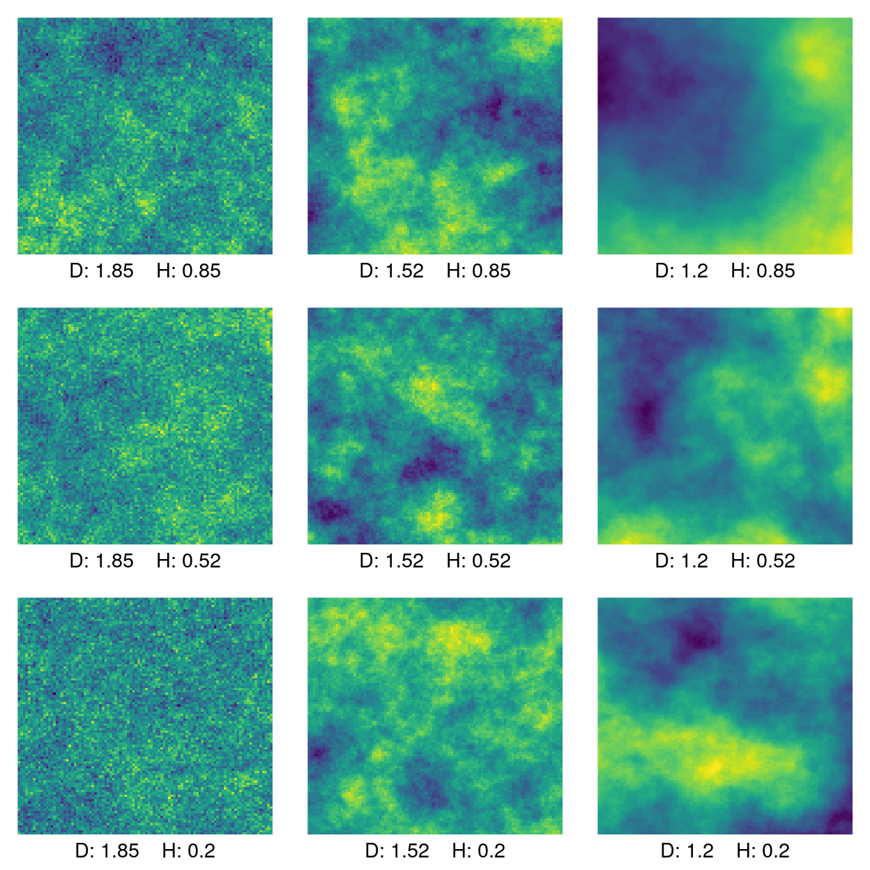
Figure 1: Cauchy process labeled by fractal dimension (D) and Hurst parameter (H).
For the above plot, fractal dimension decreases as you go to the right. The effect is pretty clear: as fractal dimension goes down the value of the functions changes more smoothly. The graphs in the first column with high fractal dimension look like static. In fact, for many practical estimators of fractal dimension, random noise has a maximal fractal dimension of 2.
The effect of the Hurst parameter is a little more subtle. A higher Hurst parameter corresponds to a higher long-range dependence. The highest Hurst parameter is 0.8 along the top row. A high fractal dimension obscures the effect of the Hurst parameter but even in the top left plot and results in some clumping of similar values. This can be compared to the high fractal dimension, low Hurst plot in the lower left, where there is very little clustering of values.
Relation to ACF
Another way to see the effect is by looking at the cross sections. Each of the following graphs is a vertical slice from each of the corresponding random fields above.
par(mfrow = c(3,3), mar = c(2,1,1,1))
plot_transects <- function(k){
  plot(
       xs[[k]][, 10],
       col = viridis::viridis(10)[3],
       type = 'l',
       lwd = 1.6,
       axes = FALSE
       )
  add_text(k)
}

# plot transects
out <- lapply(1:9, function(k) plot_transects(k))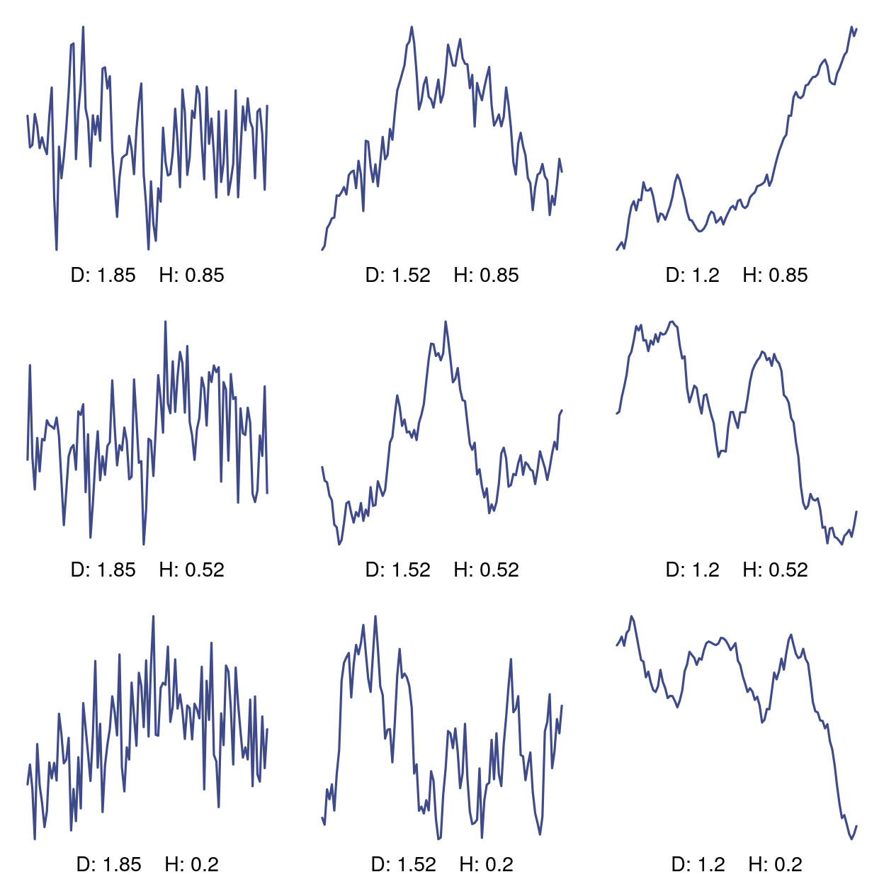
Figure 2: Cross sections of 2D Cauchy process.
Given the relation of fractal dimension to the autocorrelation function(ACF), we should see the difference in the empirical ACF of each of these time series. The effect of the Hurst parameter is a little hard to discern but in the left row with constant fractal dimension 1.85, the ACF shows less dependence on past values as the Hurst parameter decreases.
par(mfrow = c(3,3), mar = c(2,1,1,1))
out <- lapply(xs, function(x) acf(x[, 1], plot = FALSE)) %>%
lapply(., plot, yaxt = 'n') 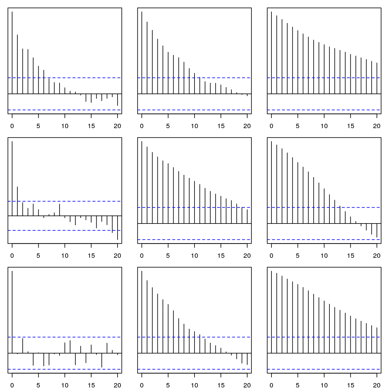
Figure 3: Autocorrelation function for lags h = 0-20
Below is a plot of the values of a fractal dimension estimator against the Hurst parameter for each of the previous time series. The plot looks somewhat like the parameter grid because changes in the Hurst parameter aren’t affecting the fractal dimension estimator. (The plot matches the functions above when rotated 90 degrees counter-clockwise.)
# Compute fractal dimension
fractal_dim <- function(x) {
  res <- fractaldim::fd.estimate(x, methods = "variogram")
  res$fd
}

transects <- lapply(1:9, function(k) xs[[k]][, 10])

plot(coeffs[, 2], lapply(transects, fractal_dim),
            pch = 15,
            cex = 1.7,
            col = viridis::viridis(10)[3],
            xlab = "Hurst Parameter",
            ylab = "Fractal Dimension Estimate")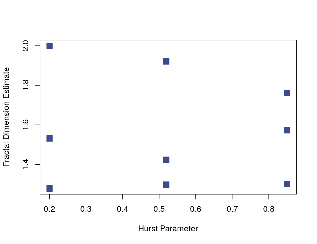
Simulations
Fractal dimension can be a useful feature for the classification or clustering of time series. Here is a simple demonstration of the ability of fractal dimension to discriminate between related ARMA processes. Naturally, whether fractal dimension is useful in other contexts depends on whether the time series or random fields in question have the kind of variation in fine scale behavior captured by fractal dimension estimators.
For these tests, I generated 50 time series of an ARMA process. The moving average(MA) component has a random element so each time series will be unique. Only the autoregressive parameters were varied for each time series.
set.seed(1)
reps = 50
t3 <- replicate(reps, arima.sim(n = 500, list(ar = c(0.5, -0.2), ma = c(-5, 0, 5))))
t2 <- replicate(reps, arima.sim(n = 500, list(ar = c(0.8, -0.2), ma = c(-5, 0, 5))))
t1 <- replicate(reps, arima.sim(n = 500, list(ar = c(1.1, -0.2), ma = c(-5, 0, 5))))

ts_list <- list(t1, t2, t3)
pal = viridis::viridis(50)[c(2, 25, 45)]

# Sample plot of each function
plot_ts <- function(k){
  plot(
        ts_list[[k]][1:250, 10],
        type = 'l',
        lwd = 1.7,
        cex = 1.6,
        bty = "n",
        yaxt = "n",
        xaxt = "n",
        xlab = paste0("Sim ", k),
        col = pal[k]
        )
}
par(mfrow = c(3,1), mar = c(4,1,1,1))
plot_ts(1); plot_ts(2); plot_ts(3)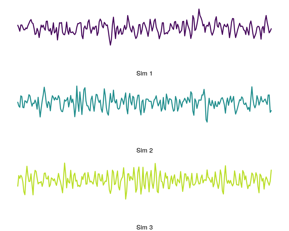
Figure 4: Sample from each group ARMA simulations.
Fractal Dimension Estimators
The R fractal dimension package has a number of estimators of fractal dimension. In a paper that accompanies the package, Gneiting et al. compare the robustness of the fractal dimension estimators, which include estimators based on box-counting dimension, wavelets, and spectral density.
They find the variogram or madogram estimators perform best. The increments of a random process are defined \((X(t) - X(t+h))\), and the variogram is the squared expectation of the increments: \[ \gamma(h) = \frac{1}{2}E\left(X(t) - X(t + h)\right)^2. \] The slope of the \(\log-\log\) regression of the variogram to the interval \(h\) determines the fractal estimator. The madogram estimator is calculated in the same way but with the absolute value of the increments used instead of the squared value.
Here’s how the fractal dimension estimate separates samples from our three simulations.
library(ggplot2)

# Compute features on each group
df1 <- apply(t1, 2, fractal_dim) %>% data.frame
df2 <- apply(t2, 2, fractal_dim) %>% data.frame
df3 <- apply(t3, 2, fractal_dim) %>% data.frame

fd_df <- rbind(df1, df2, df3)
fd_df$id <- as.factor(
                      c(rep("Sim 1", reps),
                        rep("Sim 2", reps),
                        rep("Sim 3", reps))
                        )

data_long <- reshape2::melt(fd_df, id.vars = c("id"))

ggplot(data_long, aes(x = value, fill = id)) +
       geom_density(
                alpha = 0.6,
                aes(y = ..density..),
                position = "identity",
                color = NA) +
       scale_fill_manual(values= pal) +
       xlab("Fractal Dimension") +
       ylab("") +
       theme_minimal() +
       theme(
             panel.grid = element_blank()
) 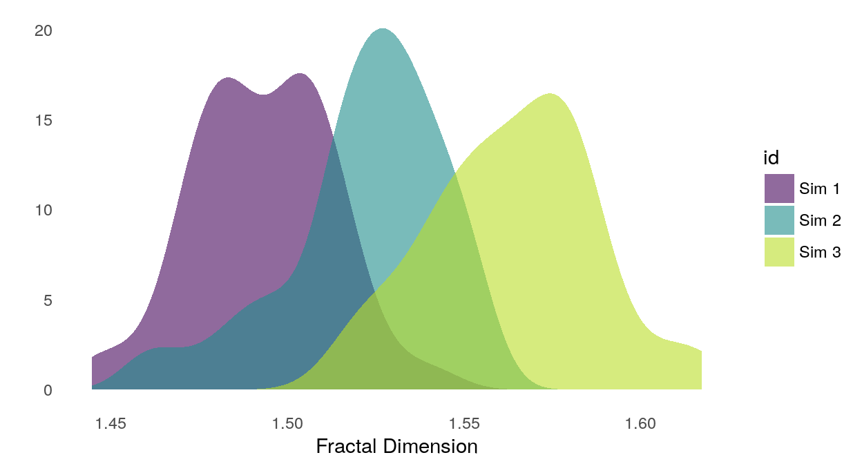
Figure 5: Smoothed density of fractal dimension estimates for each simulation group.