Exploring the Lego dataset with SQL and dplyr, part II

What we’ll do

• Query our database using dplyr
• Use dplyr functions to perform simple joins and transformations
• Create several visualizations of the use of color in Lego sets with ggplot

Other resources

• A short Rstudio introduction to dplyr.
• This Data Carpentry tutorial gives an introduction to using dplyr with SQLite and jumps directly into using dplyr syntax.
• A thorough introduction to ggplot and another ggplot primer.

Connect to the database

First we connect to the database created in the previous post. You can pass your username and password in plain text or use the keyringr package as described in the previous post.

Note: You can also run most of this code using the CSV files directly. To do this replace calls to a specific table with the corresponding dataframe loaded directly from the CSV file.

library(RPostgreSQL)
library(dplyr)

# Suppress warnings for this session
options(warn=-1)

# Set driver and get connection to database
pg = RPostgreSQL::PostgreSQL()
# Replace user and password with your value
con = DBI::dbConnect(pg, 
                user = "postgres", 
                password = keyringr::decrypt_gk_pw("db lego user postgres"), 
                host = "localhost", 
                port = 5432
                )

In the previous post I wrote a function to get the basic schema of our tables. Here I use DBI functions to examine what tables we have and what fields there are.

# Check data
DBI::dbListTables(con)
DBI::dbListFields(con, 'sets')

You can also glance at the fields in a table without loading the table into memory using dplyr. With dplyr we call a specific table with the tbl function and then manipulate the object dplyr returns and treat that object (for a limited set of functions) as if it were a dataframe.

# Example without using the pipe operator
# Get the 'sets' table
res <- tbl(con, 'sets') 
head(res, 5)

# Using pipes 
con %>% tbl('sets') %>% head(10)
# Head with default arguments
con %>% tbl('inventories') %>% head
con %>% tbl('colors') %>% head

We can also send regular SQL queries using the sql function.

res <- tbl(con, sql("select name, year from sets"))
res
dim(res)

If you notice there is something different about the output when printing the res object returned by our query. It isn’t in memory and the dim function doesn’t return the number of rows. Similar to using dbFetch, you have to tell dplyr to return the results using collect.

# Collect data
res <- tbl(con, sql("select name, year from sets")) %>% collect
res

## # A tibble: 11,673 x 2
##                            name  year
##  *                        <chr> <int>
##  1              Weetabix Castle  1970
##  2            Town Mini-Figures  1978
##  3   Castle 2 for 1 Bonus Offer  1987
##  4           Space Mini-Figures  1979
##  5           Space Mini-Figures  1979
##  6           Space Mini-Figures  1979
##  7           Space Mini-Figures  1979
##  8          Castle Mini Figures  1978
##  9 Weetabix Promotional House 1  1976
## 10 Weetabix Promotional House 2  1976
## # ... with 11,663 more rows

dim(res)

## [1] 11673     2

Now a regular in-memory tibble is returned and it can be treated as a regular object.

If we have not called collect we can examine the SQL query using show_query. Here we compare how dplyr translates a query into SQL.

res <- tbl(con, sql("select name, rgb from colors"))
show_query(res)
res <- con %>% tbl('colors') %>% select(name, rgb) 
show_query(res)

Exploring the data

Now we’re ready to explore the data a little more. With what we already have done we can look at how the number of sets changed over time. Here’s a simple bar chart showing the trend. We can just look at the count years in the ‘sets’ table.

years <- tbl(con, sql("select year from sets")) %>% collect
hist(years$year, 
      col = "gray30", 
      lwd = 2, 
      cex = 0.9,
      border = "white", 
      xlab = "Year",
      main="Lego sets per year, 1950-2017")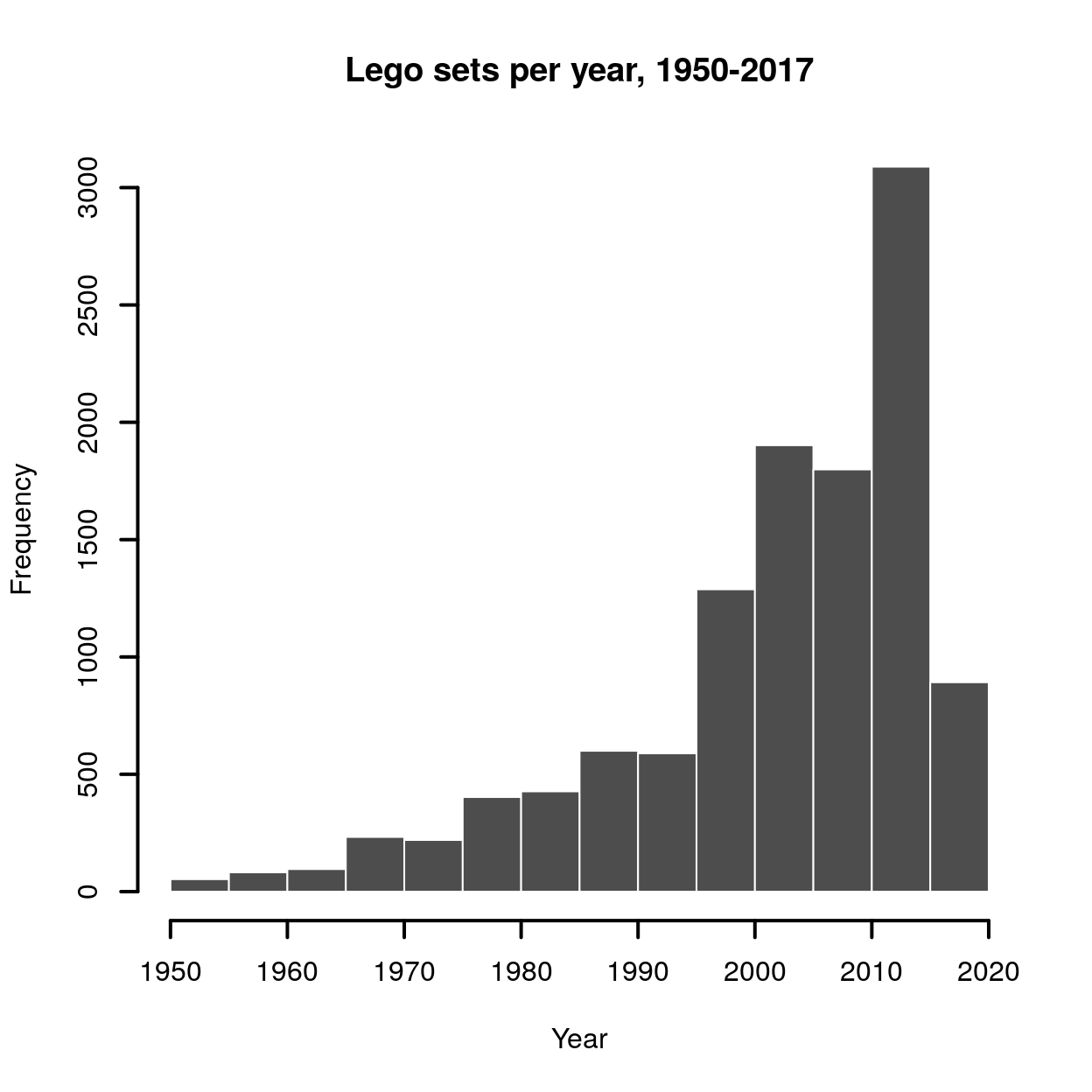

We can make a similar plot with the ggplot2 package. If you’re not familiar with ggplot, most of work is done by the first line: years %>% ggplot( ) + geom_bar(aes(x = year )) is enough to make the plot. The ggplot plot is formed by adding aesthetic layers. To make a simple bar plot we just need to add the geom_bar aesthetic and specify the variable x which determines that categories of the frequency bins.

library(ggplot2)
gp <-  years %>%  ggplot( ) + geom_bar(aes(x = year )) + 
          labs(
            x = "", 
            y = "Set count", 
            caption = "rebrickable.com/api/",
            title ="Lego sets per year, 1950-2017"
            ) +
          scale_fill_manual(values = "gray10")+ 
          theme_light( ) + 
          theme(
            panel.background = element_rect(fill = "#fdfdfd"),
            plot.background = element_rect(fill = "#fdfdfd"),
            legend.position = "none", 
            text = element_text(
                     color = "gray10", 
                     face = "bold",
                     family="Lato", 
                     size = 13),
            axis.title = element_text(size=rel(0.9)),
            plot.title = element_text(face = "bold", size = rel(1.1)),
            plot.caption = element_text(
                             face = "italic",
                             color = "gray30",
                             size = rel(0.6)),
            panel.grid = element_blank()
            )
gp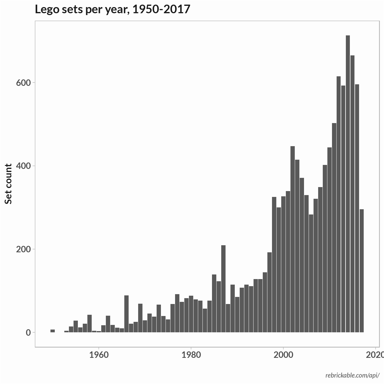

I’ll be using the same basic bar plot for the remaining plots. To simplify, we can put the extra theme modifications in a function – basically, it’s a quick a dirty way to define a theme.

theme_light2 <- function(){
  theme_light( ) + 
    theme(
          panel.background = element_rect(fill = "#fdfdfd"),
          plot.background = element_rect(fill = "#fdfdfd"),
          legend.position = "none",
          text = element_text(
                   color = "gray10", 
                   face = "bold",
                   family="Lato", 
                   size = 13),
          plot.title = element_text(size = rel(1)),
          axis.title = element_text(size=rel(0.9)),
          plot.caption = element_text(
                           face = "italic",
                           color = "gray30",
                           size = rel(0.7)),
          panel.grid = element_blank()
          )
 }

Database schema and joins

To look at how the color of Lego bricks changed over time, we will need to combine data from the different tables. For example, if we want to look at the change in colors over time we’ll need data from multiple tables. The schema below is included in the Kaggle data set. The schema shows the foreign key constraints which we’ll use to join data from the multiple tables.

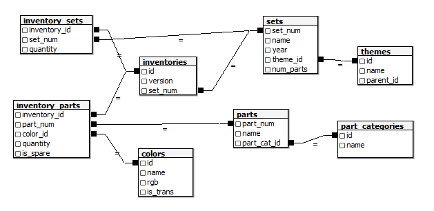
Original Lego Database Schema

For the first plot we’ll look at the frequency of brick colors per year. We’ll plot one count for each time a color showed up in a Lego set. To do this we need to join ‘sets’ with the parts in ‘inventories’, with the part id in ‘inventory_parts’, with the parts color in ‘colors’. I’m going to use a join on matching keys. In dplyr, if you are matching on columns with the same name the column with the call right_join(tbl1, tbl2, by=col_name. For some tables our column names don’t match so we name them like so: by = c("col_name1" = "col_name2").

First I’ll test a query to a single lego set to see check if the query is getting all the parts. There are two related tables – ‘inventories’ and ‘inventory_sets’ and it wasn’t clear what the role of each table was. Here I test out the query using the ‘inventories’ table and filter the ‘Space Mini-Figures’ set.

# Get table 
inventories     <- tbl(con, "inventories")
inventory_parts <- tbl(con, "inventory_parts")
colors          <- tbl(con, "colors")
sets            <- tbl(con, "sets")

# Get inventory parts for one set
sets %>% head

## # Source:   lazy query [?? x 5]
## # Database: postgres 9.3.17 [postgres@localhost:5432/postgres]
##   set_num                       name  year theme_id num_parts
##     <chr>                      <chr> <int>    <int>     <int>
## 1    00-1            Weetabix Castle  1970      414       471
## 2  0011-2          Town Mini-Figures  1978       84        12
## 3  0011-3 Castle 2 for 1 Bonus Offer  1987      199         2
## 4  0012-1         Space Mini-Figures  1979      143        12
## 5  0013-1         Space Mini-Figures  1979      143        12
## 6  0014-1         Space Mini-Figures  1979      143        12

one_set <- sets %>% filter(set_num == "0012-1") %>% 
           right_join(inventories, by = 'set_num', copy = TRUE) %>%
           right_join(inventory_parts, by = c('id' = 'inventory_id')) %>%
           filter(!is.na(year)) %>% collect  
one_set$part_num

## [1] "3626apr0001" "3838"        "3842a"       "3962a"       "970c00"     
## [6] "973p90c02"

The data come from Rebrickable and we can check to se if our result matches theirs. Here are the parts they list for the set:

Space Mini-Figures Set(1979)

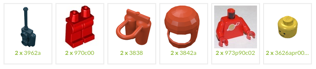
The parts match but we don’t have a single row per item since the quantity column stores the number of parts. If we wanted to get the true frequency we could expand the data set to have a row per piece.

As far as the ‘inventory_sets’ table goes, it isn’t clear what role it plays but the inventories table appears to cover the majority of the sets.

Now we can repeat the above query on all sets by removing the filter. I also added the join to add colors to each part row and selected a subset of the columns.

set_colors <- sets %>%   
              select(set_num, name, year) %>% 
              right_join(inventories, by = 'set_num', copy = TRUE) %>%
              right_join(inventory_parts, by = c('id' = 'inventory_id')) %>%
              filter(!is.na(year)) %>%
              left_join(colors, by = c('color_id'  = 'id')) %>%
              mutate(name = name.x) %>% 
              select(set_num, name, year, color_id, rgb, is_trans) %>% 
              collect

Since we won’t need to make another query we also need to close our database connection.

DBI::dbDisconnect(con)

To plot the frequency of colors of unique parts we can use most of the plot from above. We make two changes:

1. Create a set of breaks to determine x-axist ticks on every 10 years
2. Create a palette that matches the colors in the rgb column

To do the latter, we can simply use the rgb for the palette and add a name so that ggplot will match the name to the color.

# Make hex values readable by R
breaks <- seq(1950, 2017, by = 10)

# Create color pallete and add names. 
set_colors <- set_colors %>% mutate(rgb = paste0("#", rgb))
pal <- unique(set_colors$rgb)
names(pal) <- unique(pal) 

gp <-  set_colors %>%   ggplot() + 
          geom_bar(aes(x = year, fill = rgb)) + 
          labs(
            x =   "", 
            y = "Brick Color Frequency", 
            title = "Lego brick colors, 1950-2017", 
            caption = "source: rebrickable.com/api/"
            ) +          
          scale_fill_manual(values = pal) + 
          scale_x_discrete(limits = breaks) +          
          theme_light2() 

gp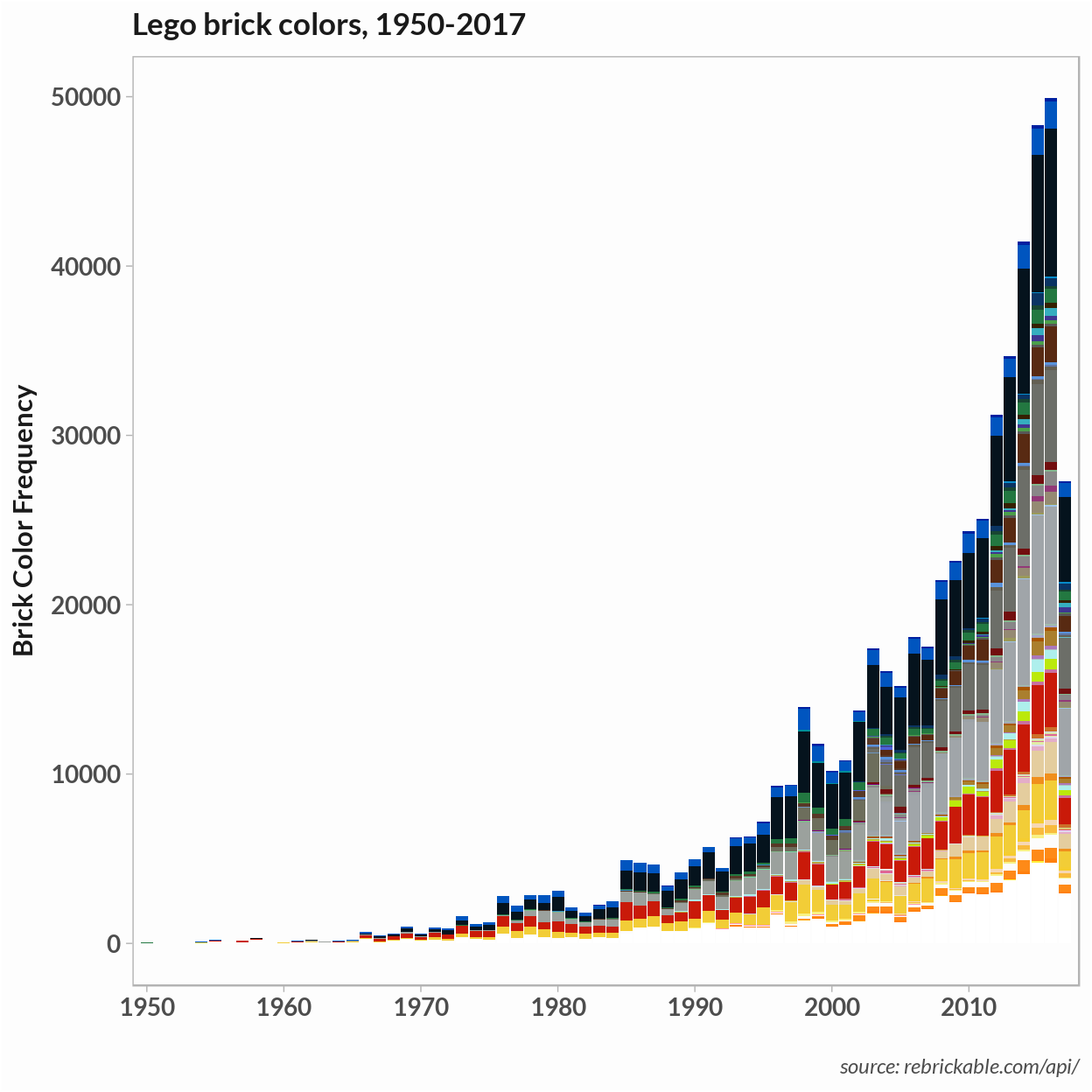

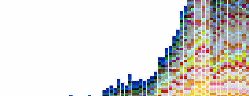
Finally, we can use dplyr’s group_by function count the number of times a color appears each year. We can use the same table to plot the occurrences of unique colors and the relative frequency of colors.

# Get number of occurences and frequency of color
freq_tbl <- set_colors %>% select(year, rgb, color_id) %>% 
              group_by(year, rgb) %>%
              summarise(n = n()) %>% 
              mutate(percent = n/sum(n))

# Plot color occurences only
gp <-  freq_tbl %>%   ggplot() + 
          geom_bar(aes(x = year, fill = rgb)) + 
          labs(
            x = "", 
            y = "Unique Brick Colors", 
            title = "Lego brick colors, 1950-2017",
            caption = "source: rebrickable.com/api/"           
            )  +          
          scale_fill_manual(values = pal)+ 
          scale_x_discrete(limits = breaks) +          
          theme_light2()

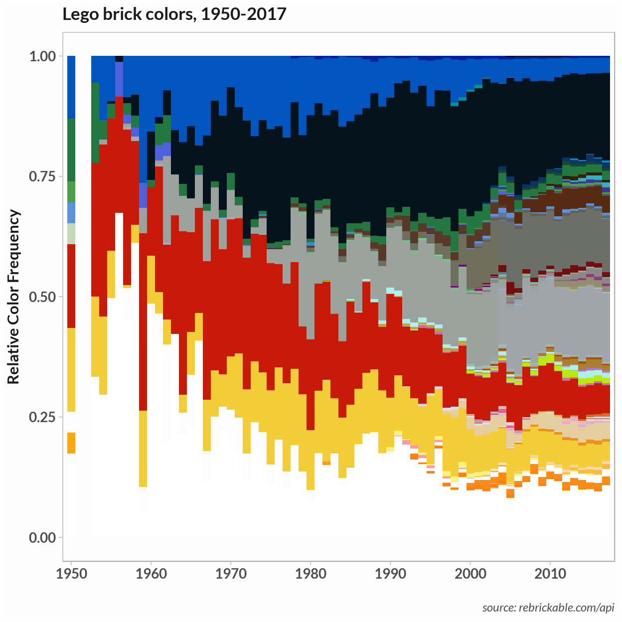
gp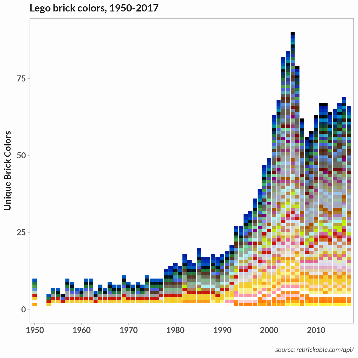

To plot relative color frequencies that we calculate above, we just add y = percent to the geom_bar aesthetics.

gp <-  freq_tbl %>% ggplot() + 
        geom_bar(
          aes(x = year, y = percent, fill = rgb), 
          stat  = "identity", 
          width = 1
          ) +
        labs(x = "", 
          y = "Relative Color Frequency", 
          title = "Lego brick colors, 1950-2017",
          caption = "source: rebrickable.com/api") +
        scale_fill_manual(values = pal) + 
        scale_x_discrete(limits = breaks) +          
        theme_light2()

gp