Exploring the Lego dataset with SQL and dplyr

What we’ll do

• Get an introduction to the DBI interface
• Create a Postgres database
• Import tables from CSV files
• Use a few simple SQL queries
• Make a simple plot of the data

Related Tutorials

• This Data Carpentry tutorial gives an introduction to using dplyr with SQLite and jumps directly into using dplyr syntax.

• This UseR2017 talk by Barbara Borge Ribeiro give a quick overview of programmatically accessing relational databases from R

• Software Carpentry has a introductory tutorial for using databases and SQL which includes lessons for Python and R here.

• RStudio has a nice overview of database related packages here, which includes a history of the the DBI interface.

Setup and download

In addition to dplyr and RPostgreSQL, we will use the readr package was has an enhanced method for reading CSV files. Throughout the code I will be using the :: operator to identify the namespace R searches for function calls from these packages. Calling functions this way avoids the need to load a package using library() or require(), and it makes explicit what package individual functions come from. The exception is the pipe operator %>% which I use the import package to make available to the current session.

# library("dplyr")
# library("RPostgreSQL")
# library("readr")
# library("import") 
library(DBI)
import::from(dplyr, "%>%")

First, we need to create a project directory – I’ll be calling it ‘lego-project’ – and set your current directory to that folder. There are a lot of unhelpful warnings so I’m suppressing those for the session by setting the option options(warn=-1). You can skip this line if you’d like to see all the warnings.

setwd("~/path/to/my/lego-project")
# Supress warnings for this session
options(warn=-1)

We’ll download the zip to a temporary file and save the CSV files to the data directory.

URL <- "https://s3-us-west-1.amazonaws.com/kaggle-lego/lego-database.zip"
tmp <- tempfile()
download.file(URL, tmp)
dir.create("data")
# Unzip files in the data directory
setwd("data")
files <- unzip(tmp)

Check out the data

Now we should have the CSV files unzipped and the file names in files. If you look at the files you’ll see it includes 8 CSV files and one image named downloads_schema.png. This contains the schema for the database the files came from. This details primary and foreign keys and constraints which we won’t be using here. The schema will come in handy in the next tutorial, however, when we need to join data from multiple tables.

For now we remove it from the files list and grab the filenames for later use. If you have not used the pipe function %>%, imported from dplyr, it sends output from the left-hand function to the right-hand function. The . is a placeholder argument representing the values output by the left-hand function.

# Check files names
files 
# Remove db schema '.png' file
files <- files[-2]
# Remove file prefix and suffix 
filenames <- files %>% sub("./", "", .) %>% sub(".csv", "", .) 

Here we glance at the first few rows of the data. Several featurs make it a nice alternative to the base read.csv function: read_csv reports the data type of each imported column; It also does not convert strings to factors by default, i.e., stringsAsFactors = FALSE. The result of the function is a tibble which can be treated as a data.frame. Glancing at the head() of the tibble will also report column types.

# Glance at head of color
readr::read_csv(files[1], n_max = 5)
# Look at heads of all files
lapply(files, readr::read_csv, n_max = 5)

For a larger dataset, it might also be useful to check the number of rows of data. I’m going to use the system function to make a call to wc. The system function allows you to pass command line function to the operating system, so it is OS dependent. These commands should work on Linux or macOS and is an efficient way to get the newline count of a file. I’ll turn this into a function so we can use lapply to iterate over the files. (I’ve commented out a similar function for Windows but I haven’t tested that function.)

# For Linux/Unix or Mac
count_rows <- function(filename){
  system(paste("wc -l", filename))
}
out <- lapply(files, count_rows)
# For Windows (did not test)
# count_rows <- function(filename){
#  system(paste("nd /c /v 'A String that is extremely unlikely to occur',
#        filename))

At this point, we have an overview of the data types and size of each file. The data are either integers or strings. One possibility would be to update, for example, the is_trans field in colors to be a boolean or logical data type. To keep it simple we will be importing the data types as is.

Create the database

Now we have checked out all the ingredients ready can create our database. You’ll need a working installation of Postgres and the username and password for an account. The following db functions are from the RPostgreSQL(and DBI) package.

In this example, we’ll use your password as plain text in the script. This isn’t the best practice and I give an alternative below.

First, we identify the database driver we’ll be using and setup the connection, con, which we can use both create and query the database. To use another database, only the first line would need to be changed. If you already had SQLite installed, for example, just load the RSQLite packages and call the analagous function to retrieve the SQLite driver. The remaining DBI calls should work, give or take variations in SQL syntax.

# Access Postgres driver 
pg = RPostgreSQL::PostgreSQL()
# Note fake user/password
con = DBI::dbConnect(pg, 
                     user = "my-username", 
                     password = "#my-password", 
                     host = "localhost", 
                     port = 5432
                     )

If all has gone well we now have a connection to the Postgres and can create our database. With the dbSendStatement command we can use any standard PostgreSQL command. We create the database with “create database legos”. and then test use the dbReadTable to create tables. For each CSV file, we create a single table using the filenames we created earlier.

DBI::dbSendStatement(con, "create database legos")
# Test writing one file to the database
colors <- readr::read_csv(files[1])
DBI::dbWriteTable(con, "colors", colors , row.names=FALSE)
# Check that it works
dtab <- DBI::dbReadTable(con, "colors")
summary(dtab)
# Write all files to the database
for(k in seq_along(files[1:8])){
  cat("Writing ", filenames[k], "/n")
  tmp <- readr::read_csv(files[k])
  DBI::dbWriteTable(con, filenames[k], tmp, row.names=FALSE)  
  rm(tmp)
}
dtab <- DBI::dbReadTable(con, "sets")
summary(dtab)
# Close connection
DBI::dbDisconnect(con)

At this point, our database has been created and we’re ready to do some analyses. If we were creating a database which we’d be adding more rows to in the future it would be good to define key constraints or specify our column types in more detail.

Interlude: Password encryption with keyringr

(If you start a new session you can pick up again here. If continuing with the previous analysis, you can skip the code in this section and still run the rest of the tutorial.)

There is a nice alternative to using plain text passwords in scripts. The keyringr package lets you encrypt your passwords locally and call those passwords from a script. The package provides three separate functions for doing this and which you should use depends on your operating system. I will use the Linux function below. See the instructions here for a quick guide to the package and the function calls for different operating systems.

If you have started a new session you can resume at this point. In the code below I assume that we have created the database and reconnecting to the database with a fresh R session.

For the password argument passed to the dbConnect function below, you will need to replace keyringr::decrypt_gk_pw("db lego user myusername") with the keyringr decryption function that’s appropriate for your operating system. Also, you need to replace the key-value pairs, here db lego and user myusername with those passed you used to set up your encrypted password.

# If restarting, re-set the directory to data
setwd("~/path/to/my/lego-project")
# Get filenames again
filenames <- dir() %>% sub(".csv", "", .)
install.packages("keyringr")

# Replace plaintext password with keyringr call
pg = RPostgreSQL::PostgreSQL()
con = DBI::dbConnect(pg, 
                user = "postgres", 
                password = keyringr::decrypt_gk_pw("db lego user myusername"), 
                host = "localhost", 
                port = 5432
                )

Note: The keyring package serves the same purpose and is available for installation using devtools.

Checking the database schema

We retrieved two tables above to verify that they had been created. It would be nice to verify all the tables were created and to check the database’s current schema. Since we have a list of the table names, we’ll create a function that takes the table names so we can loop over the functions with lapply.

The information schema is a set of views containing information about the database, user roles, column data types and a lot more. We will query the column view to check the data type and maximum character length.

The dbSendQuery can be used for sending standard SELECT queries, (and for more genral SQL statements although it is not recommended). The command does not return data until we call the dbFetch and results must be cleared with dbClearResult.

If you have not fetched the data you’ll get an error about ‘impending rows’. Clear the list with dbClearResult(dbListResults(con)[[1]]).

# Function to check table schema
get_schema_query <- function(tab){
  paste0("select column_name, data_type, character_maximum_length", 
  " from INFORMATION_SCHEMA.COLUMNS where table_name = '",tab,"';")
}
# Check an example
res <- DBI::dbSendQuery(con, get_schema_query("sets"))
DBI::dbFetch(res)
DBI::dbClearResult(res)
# Create function from previous example
check_schemas <- function(tab){
  res <- DBI::dbSendQuery(con, get_schema_query(tab))
  out <- DBI::dbFetch(res)
  DBI::dbClearResult(res)
  out
}
# Check all tables
schemas <- lapply(filenames, check_schemas)
names(schemas) <- filenames  

For queries where you know the size of the results is not too large or in interactive contexts, dbGetQuery performs basically the same tasks as the three DBI calls used above. I’ll use this command instead of the multistep calls required by dbSendQuery below.

Let’s plot something

In the next tutorial, I’ll go over using dplyr functions to do some basic querying of the data. But we’ve made it this far so let’s plot something. We’ll query the color data set and plot all the colors used in lego sets since 1950.

Colors are stored in the rgb column and transparency in is_trans. Here we pass dbGetQuery a basic SQL select command.

# Select rgb and is_trans columns 
rgb_df <- DBI::dbGetQuery(con, "select rgb, is_trans from colors")

# Check data
dim(rgb_df)
head(rgb_df)

Both columns are of type ‘character’. The rgb colors are in hexadecimal and R will read string hexadecimals as colors. The values, however, don’t reflect the transparency. We use dplyr functions to filter rows with transparent colors and count to get the total number of rows returned by the previous step. In the next line, we add a column with the color adjusted for transparency. The ifelse statement sets the new column, named rgbt, to the straight rgb value if is_trans is false, otherwise, it adds an alpha value determined by the adjustcolor function.

rgb_df$rgb <- paste0("#", rgb_df$rgb) 
head(rgb_df)
# Count number of transparent colors
rgb_df %>% dplyr::filter(is_trans == "t") %>% dplyr::count()
# And rgb + alpha column
rgb_df <- rgb_df %>% dplyr::mutate(rgbt = ifelse  (is_trans ==  "f", rgb,adjustcolor(rgb, 0.5)))

Now we plot the results. The sort function orders the hex values alphanumerically, which isn’t a perfect color sorting but it’s not too bad either.

par(bg = "gray10", mar = c(2,1,2,1))
barplot(
        height = rep(0.5, nrow(rgb_df)), 
        col = sort(rgb_df$rgb), 
        yaxt ="n", 
        border = par("bg"),
        space = 0
        )

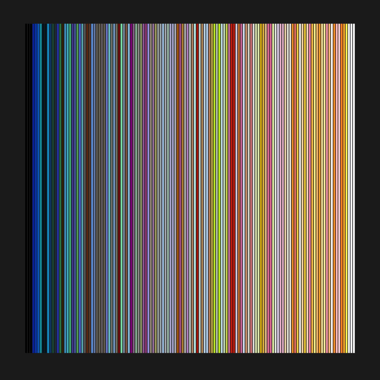
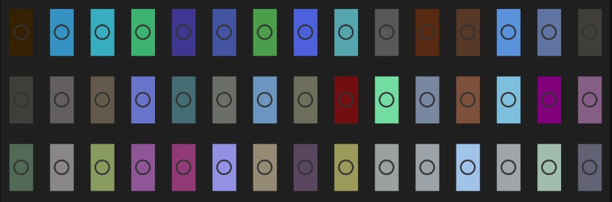
Cool, although it’s hard to tell what affect transparency has. Perhaps ploting the colors with a larger area will help identify the transparent tiles. We could also fiddle with the alpha value that’s passed to the adjustcolor() function. We’ll draw each color in a separate plot defined by the draw_lego function and adjust par to plot all 135 entries. This is good old-fashioned base R plotting.

# Draw a single square
draw_lego <- function(col){
  plot(5,5, type = "n", axes = FALSE)
  rect(
        0, 0, 10, 10, 
        type = "n", 
        xlab = "", 
        ylab = "",
        lwd = 4,
        col = col, 
        add = TRUE 
      )
  points(x = 5, y = 5, col ="gray20", cex = 3, lwd = 1.7)
  }

op <- par(bg = "gray12")
plot.new()

par(mfrow = c(9, 15), mar = c(0.7, 0.7, 1, 0.7))
cols <- sort(rgb_df$rgbt)
for(k in 1:length(cols))  draw_lego(cols[k])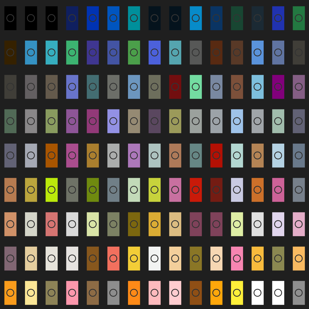

Maybe it’s a little corny, maybe you like corny; In any case, it’s good enough for a quick view of the colors.

In the follow-up post, I’ll go over using dplyr to query, filter, and transform data from our lego database. In order to explore the data in more detail, we’ll also need to do some basic joins.

Finally, for this session, we need to clean up the open connection and reset the warnings option.

DBI::dbDisconnect(con)
# Unsupress warnings
options(warn= 0)